Introduction

The film-industry is in a constant growth trend. The global box office was worth 41.7 billion in 2018. Hollywood has the world’s most massive box office revenue with 2.6 billion tickets sold and around 2000 films produced annually.

One of the main interests of the film studios and related stakeholders is a prediction of revenue that a new movie can generate based on a few given input attributes.

Background

Starting in 1929, during the Great Depression and the Golden Age of Hollywood, an insight began to evolve related to the consumption of movie tickets. It appeared that even in that bad economic period, the film industry kept growing. The phenomenon repeated in the 2008 recession.

The primary goal is to build a machine-learning based model that will predict the revenue of a new movie given such features as cast, crew, keywords, budget, release dates, languages, production companies, and countries.

EDA was the first step followed by introducing an initial linear model and comparing it to other models at the end of the process. 7398 movies data collected from The Movie Database (TMDB) as part of a kaggle.com Box Office Prediction Competition. A train/test division is also given to build and evaluate the developed model.

The Challenge

Consumer behaviours have changed over the years: the MeToo movement, as well as other social developments, have surfaced in our society, and that reflected in movie scripts. However, some of the preferences that were relevant 50 years ago are still relevant today; hence, an analysis based on the last few decades of movies production is always appropriate and will be able to serve any stakeholders that have an interest in predicting a new movie revenue.

The Packages that I used in this exercise:

import warnings
warnings.filterwarnings('ignore')
import numpy as np
import matplotlib.pyplot as plt
%matplotlib inline
import pandas as pd
from scipy import stats
from scipy import stats, special
from sklearn import model_selection, metrics, linear_model, datasets, feature_selection
from sklearn import neighbors
from sklearn.preprocessing import StandardScaler
import time
from scipy import io
from sklearn.preprocessing import StandardScaler
from sklearn.model_selection import train_test_split
from sklearn.linear_model import LogisticRegression
from sklearn.model_selection import cross_val_score, KFold
from sklearn.neighbors import KNeighborsClassifier
from sklearn.tree import DecisionTreeClassifier
from sklearn.metrics import confusion_matrix
from sklearn.model_selection import cross_validate
from sklearn.preprocessing import LabelEncoder
from vaderSentiment.vaderSentiment import SentimentIntensityAnalyzer
import json
import seaborn as sns
import ast

EDA

Pictures are best to illustrate and present first findings from the dataset. Begin the exploration with a scatter plot of ‘Revenue vs Budget’ to view the upper-end data points:

plt.figure(figsize=(8,6))
plt.scatter((train['budget']), (train['revenue']))
plt.title('Revenue vs Budget')
plt.xlabel('Budget')
plt.ylabel('Revenue')
plt.show()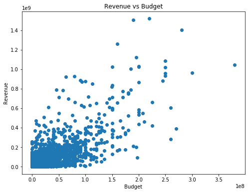

Continue the exploration with a scatter plot that will show us the lower-end points by using a log10 of the values, the plot of ‘Revenue vs Budget’ will change:

plt.figure(figsize=(8,6))
plt.scatter(np.log10(train['budget']), np.log10(train['revenue']))
plt.title('Revenue vs Budget')
plt.xlabel('Budget [log10]')
plt.ylabel('Revenue [log10]')
plt.show()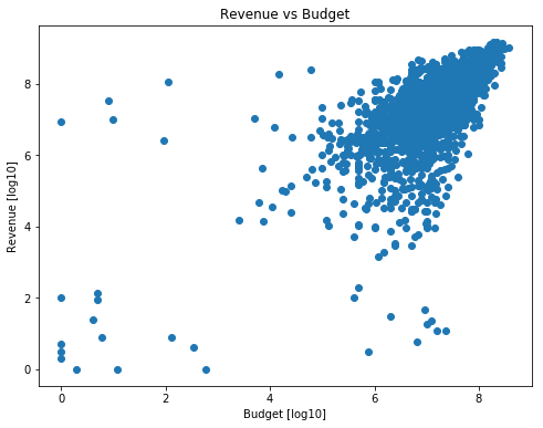

Checking the scatter plot of ‘Revenue vs Popularity’.

plt.figure(figsize=(8,6))
plt.scatter(np.log10(train['popularity']), np.log10(train['revenue']))
plt.title('Revenue vs popularity')
plt.xlabel('Popularity [log]')
plt.ylabel('Revenue [log]')
plt.show()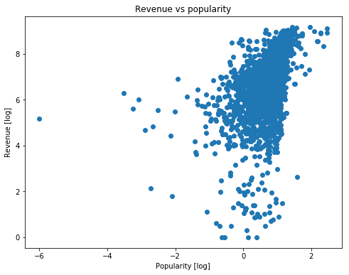

Comparing the movies with the biggest budget values:

train.sort_values('budget', ascending=False).head(10).plot(x='original_title', y='budget', kind='barh')
plt.xlabel('Budget [USD]');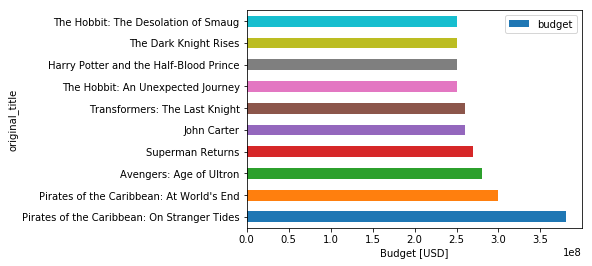

Comparing the movies with the biggest Revenue values:

train.sort_values('revenue', ascending=False).head(10).plot(x='original_title', 
                                                            y='revenue', kind='barh')
plt.xlabel('Revenue [USD]');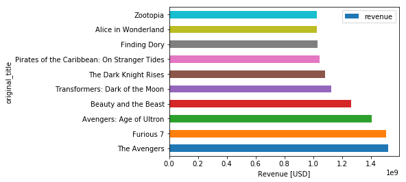

Comparing the movies with the biggest Profit values:

train.assign(profit = lambda df: df['revenue'] - df['budget'] ).sort_values('profit', 
                                   ascending=False).head(10).plot(x='original_title', 
                                                                  y='profit', kind='barh')
plt.xlabel('Profit [USD]');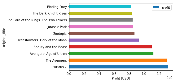

Moving ahead to explore the highest Revenue by ‘genres’ as follow:

train.groupby('genres')['revenue'].mean().sort_values().plot(kind='barh')
plt.xlabel('Revenue [USD]');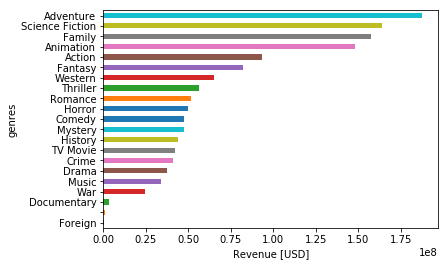

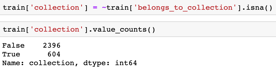
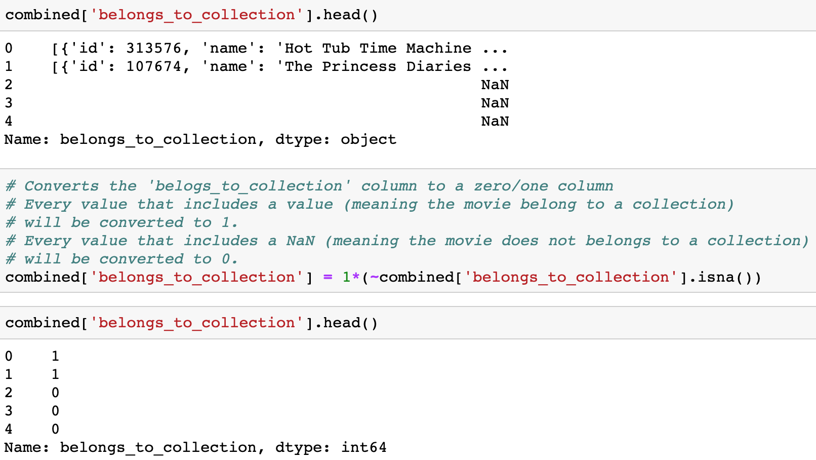
The column ‘belongs_to_collection’ was converted to a ‘True’ / ‘False’ column, if a movie belongs to a collection of movies, or not.

Simple box-plot revel that movies that belong to a collection benefit from a higher Revenue as reflected by the median and the range (25,75 percentile), the orange (right) box-plot is more elevated.

fig, ax= plt.subplots(figsize=(8,6))
ax.set_yscale('symlog')
sns.boxplot(x= 'collection', y='revenue', data=train, ax=ax);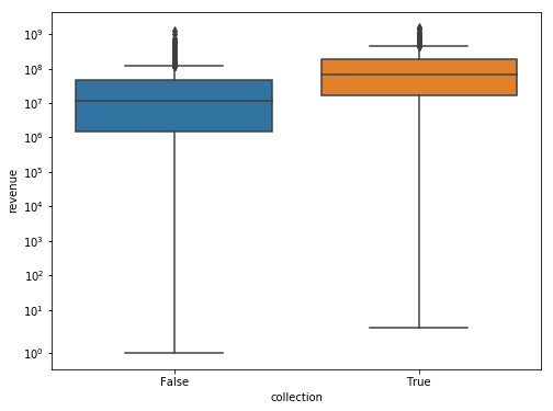

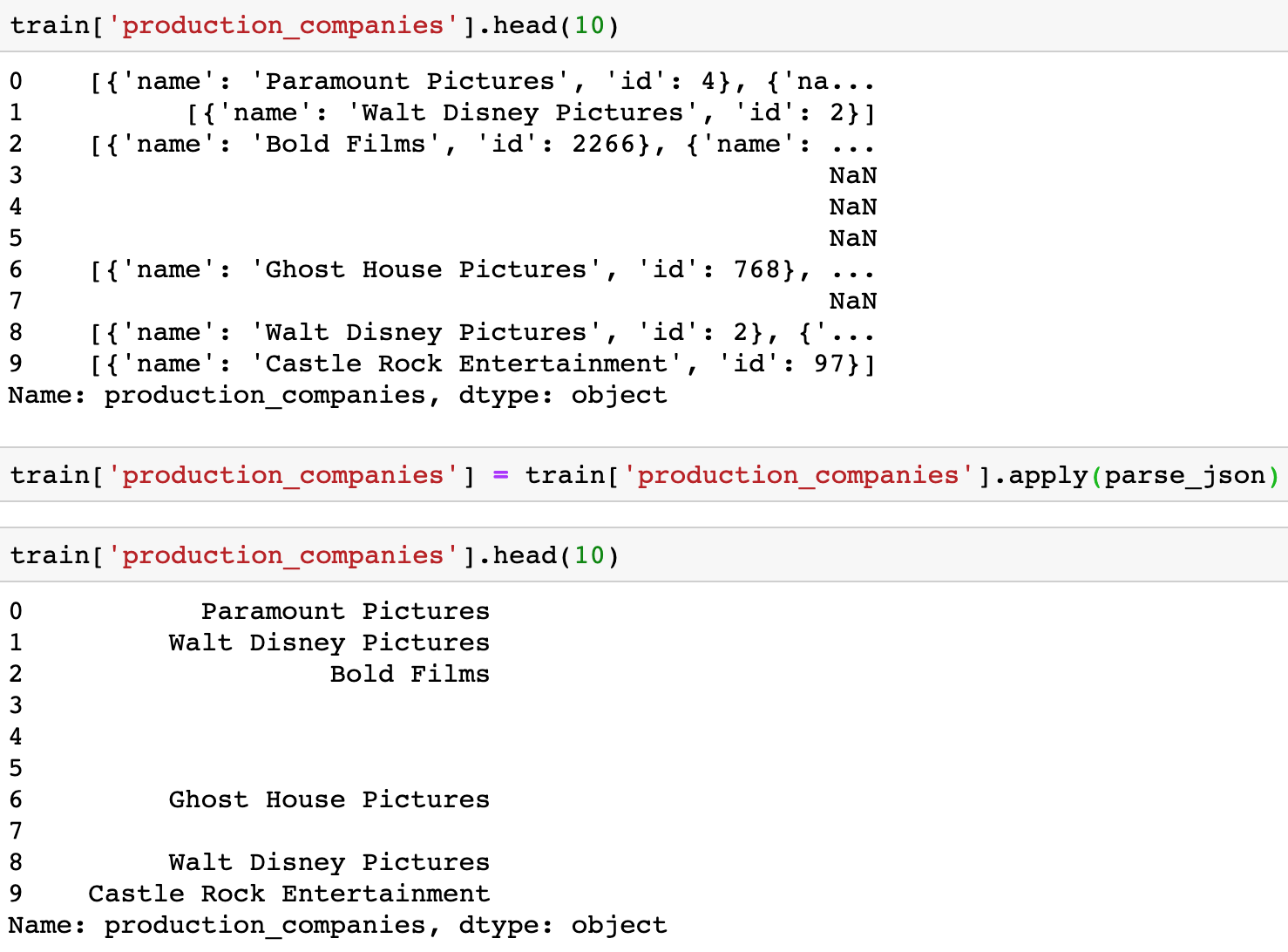
Define a function (named ‘parse_json’) to parse the first ‘name’ value from this structure of a list of dictionaries:

def parse_json(x):
    try:
        return json.loads(x.replace("'", '"'))[0]['name']
    except:
        return ''

Applying the ‘parse_json’ function on the ‘production_companies’ column yields:

Visualizing the production companies with the highest Revenue yields the plot:

train.groupby('production_companies')['revenue'].mean().sort_values(ascending=False).head(20).plot(kind='barh')
plt.xlabel('Revenue [USD]');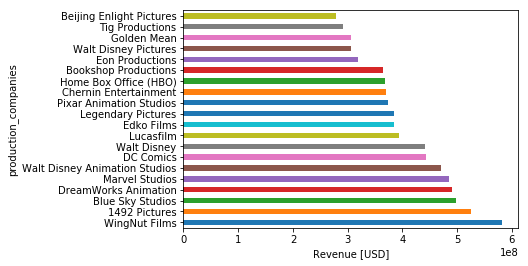

Data Preparation

Starting with Sentiment AnaLysis of the columns ‘overview’ and ‘tagline’ that contains a short verbal overview of the movie as well as the relevant tagline. I used vaderSentiment package with the value ‘compound’ to explore the question: Does a sentiment analysis is correlated with the Revenue column?

# using SentimentIntensityAnalyzer function from the vaderSentiment package
# for an analysis of the sentiment of the films 'overview' and 'tagline'
analyser = SentimentIntensityAnalyzer()

# Fill out the NaNs values in 'overview' and 'tagline'
# with an empty string ('') before processing the analyser scores
train['overview'] = train['overview'].fillna('')
train['tagline'] = train['tagline'].fillna('')

# As we can see from the sentiment analysis, there is (almost) no correlation between
# the 'compound' value generated by vaderSentiment package (a composition sentiment value)
# To the 'overview' and 'tagline' columns.
train[['tag_sentiment', 'sentiment']].corrwith(train['revenue'])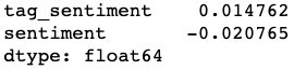

Continue with a helper function that helps to convert the given data as string to a list, for example, the function will convert ‘[1,2,3,4]’ (string) into [1,2,3,4] (a list).

# Helper function to parse text and convert given strings to lists 
def text_to_list(x):
    if pd.isna(x):
        return ''
    else:
        return ast.literal_eval(x)

The next step is to combine the Train and Test Sets into a combined Set, all the preparations will be done on the combined Set that will be split later.

combined = pd.concat((train, test), sort=False)

Drop all of the not-relevant columns from the combined dataset Columns that will not contribute to predicting the revenue.

combined.drop(columns=['id','imdb_id', 'poster_path', 'title', 'original_title'], inplace=True)

Preparation for the parsing step, applying ‘text_to_list’ function on the relevant columns.

for col in ['genres', 'production_companies', 'production_countries', \
            'spoken_languages', 'Keywords', 'cast', 'crew']:
    combined[col] = combined[col].apply(text_to_list)

Converts the ‘belogs_to_collection’ column to a zero/one column. Every value that includes some value (meaning the movie belong to a collection) will be converted to 1. Every value that includes a NaN (meaning the movie does not belong to a collection) will be converted to 0.

Reminder, a Sentiment analysis Revealed that there is no correlation between the columns: ‘overview’ and ‘tagline’ to the ‘revenue’ column. (our predicted column) Hence, we will create a binary label for each movie ‘tagline’ (and for ‘homepage’ as well later), for every movie: has or has not a ‘tagline’ and a ‘homepage’. The second step will be to create a new feature with an overview of characters count.

combined['tagline'] = 1*(~combined['tagline'].isna())
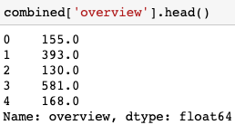
combined['homepage'] = 1*(~combined['homepage'].isna())

Creating a new feature, the new feature includes the number of characters in each movie’s overview.

# New feature includes the number of characters in each movie's overview
combined['overview'] = combined['overview'].str.len()
# Any movie without an overview (Nan) will set to zero
combined['overview'].fillna(0, inplace=True)

The head() of the new feature:

Creating a new feature contains the NUMBER of genres for each movie.

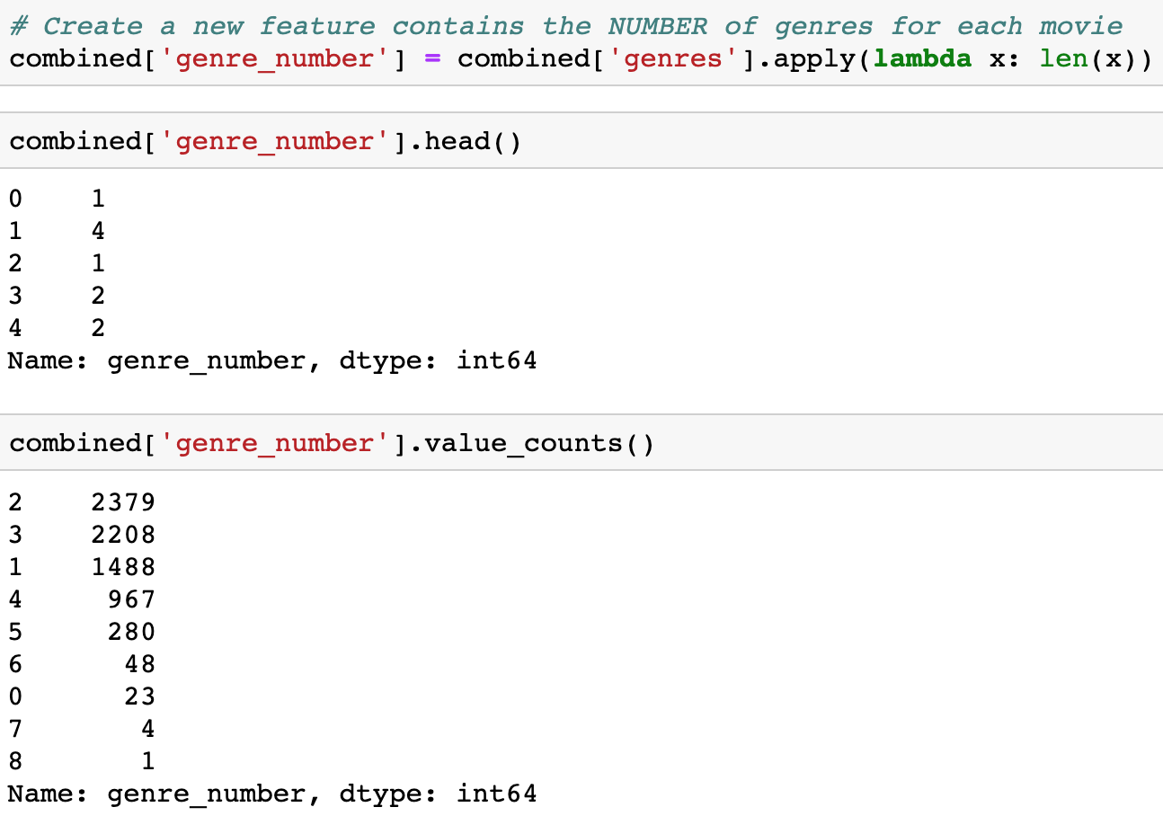
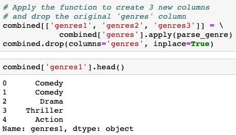
Moving on to parse the ‘genres’ names from the ‘genres’ column. Some movies have more than one genre while others have no genre at all. For this purpose, there is a helper function named: ‘parse_genre’ that will parse the first three genres that relates to a movie (if exists) and create 3 new columns named: ‘genres1’, ‘genres2’, ‘genres3’ in the combined dataset.

def parse_genre(x):
    if type(x) == str:
        return pd.Series(['','',''], index=['genres1', 'genres2', 'genres3'] )
    if len(x) == 1:
        return pd.Series([x[0]['name'],'',''], index=['genres1', 'genres2', 'genres3'] )
    if len(x) == 2:
        return pd.Series([x[0]['name'],x[1]['name'],''], index=['genres1', 'genres2', 'genres3'] )
    if len(x) > 2:
        return pd.Series([x[0]['name'],x[1]['name'],x[2]['name']], index=['genres1', 'genres2', 'genres3'] )

Apply the function to create 3 new columns and drop the original ‘genres’ column:

Creating a new column with the number of production companies related to each movie with the code-line:

combined['production_company_number'] = \
        combined['production_companies'].apply(lambda x: len(x))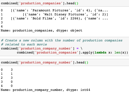

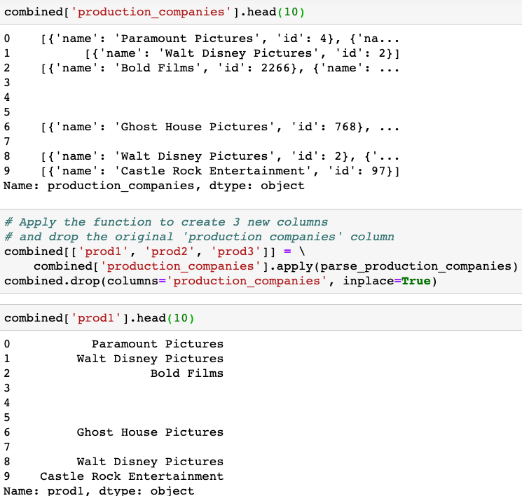
Building a function to parse the production companies of a movie. Few movies do not have a production companies value, some have more than one value, the function will parse only the first 3 production companies (if exist) and create 3 new columns named: ‘prod1’, ‘prod2’, ‘prod3’ in the combined dataset.

def parse_production_companies(x):
    if type(x) == str:
        return pd.Series(['','',''], index=['prod1', 'prod2', 'prod3'] )
    if len(x) == 1:
        return pd.Series([x[0]['name'],'',''], index=['prod1', 'prod2', 'prod3'] )
    if len(x) == 2:
        return pd.Series([x[0]['name'],x[1]['name'],''], index=['prod1', 'prod2', 'prod3'] )
    if len(x) > 2:
        return pd.Series([x[0]['name'],x[1]['name'],x[2]['name']], index=['prod1', 'prod2', 'prod3'] )

Apply the function to create 3 new columns and drop the original ‘production companies’ column.

Create a new column with the number of production countries related to each movie with the code-line:

combined['production_country_number'] = \
        combined['production_countries'].apply(lambda x: len(x))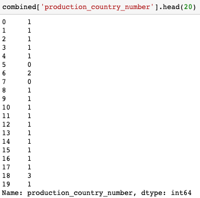

Few movies do not have a production countries value, some have more than one value. A helper function will parse the production countries of a movie. It will parse only the first 3 production countries (if exist) and create 3 new columns named: ‘country1’, ‘country2’, ‘country3’ in the combined dataset.

def parse_production_countries(x):
    if type(x) == str:
        return pd.Series(['','',''], index=['country1', 'country2', 'country3'] )
    if len(x) == 1:
        return pd.Series([x[0]['name'],'',''], index=['country1', 'country2', 'country3'] )
    if len(x) == 2:
        return pd.Series([x[0]['name'],x[1]['name'],''], index=['country1', 'country2', 'country3'] )
    if len(x) > 2:
        return pd.Series([x[0]['name'],x[1]['name'],x[2]['name']], index=['country1', 'country2', 'country3'] )

Apply the function to create 3 new columns and drop the original ‘production countries’ column with the code-line:

combined[['country1', 'country2', 'country3']] = \
                combined['production_countries'].apply(parse_production_countries)
combined.drop(columns='production_countries', inplace=True)

The ‘release_date’ column need a parse and a fill for the Nan values, that will be done with the following code:

# Parse and break-down the date column ('release_date' column)
combined['release_date'] = pd.to_datetime(combined['release_date'], format='%m/%d/%y')

# Parse 'weekday'
combined['weekday'] = combined['release_date'].dt.weekday

# fill Nan in 'weekday' column with the most common weekday value - 4
combined['weekday'].fillna(4, inplace=True)

# Parse 'month'
combined['month'] = combined['release_date'].dt.month

# fill Nan in 'month' with the most common month value - 9
combined['month'].fillna(9, inplace=True)

# Parse 'year'
combined['year'] = combined['release_date'].dt.year

# fill Nan in 'year' with the median value of the 'year' column
combined['year'].fillna(combined['year'].median(), inplace=True)

# Parse 'day'
combined['day'] = combined['release_date'].dt.day

# fill Nan with the most common day value - 1
combined['day'].fillna(1, inplace=True)

# Drop the original 'release_date' column
combined.drop(columns =['release_date'], inplace=True)

Fill the Nan values in the ‘runtime’ column with the median value.

combined['runtime'].fillna(combined['runtime'].median(), inplace=True)

Create a new column with the number of spoken languages for each movie with the code-line:

combined['spoken_languages_number'] = \
        combined['spoken_languages'].apply(lambda x: len(x))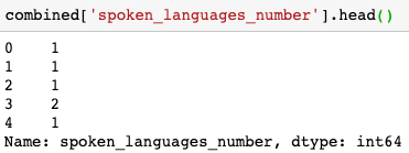

Few movies do not have a spoken languages value, some have more than one value the function. A helper function to parse the spoken languages of a movie. will parse only the first 3 spoken languages (if exist) and create 3 new columns named: ‘lang1’, ‘lang2’, ‘lang3’ in the combined dataset:

def parse_spoken_languages(x):
    if type(x) == str:
        return pd.Series(['','',''], index=['lang1', 'lang2', 'lang3'])
    if len(x) == 1:
        return pd.Series([x[0]['name'],'',''], index=['lang1', 'lang2', 'lang3'])
    if len(x) == 2:
        return pd.Series([x[0]['name'],x[1]['name'],''], index=['lang1', 'lang2', 'lang3'])
    if len(x) > 2:
        return pd.Series([x[0]['name'],x[1]['name'],x[2]['name']], index=['lang1', 'lang2', 'lang3'])

Apply the function to create 3 new columns and drop the original ‘spoken languages’ column:

combined[['lang1', 'lang2', 'lang3']] = \
            combined['spoken_languages'].apply(parse_spoken_languages)
combined.drop(columns='spoken_languages', inplace=True)

Most of the ‘status’ column values are ‘Released’, hence, the Nan values in this column will change to ‘Released’.

combined['status'].fillna('Released', inplace=True)

Create a new column with the number of Keywords for each movie.

combined['keywords_number'] = \
        combined['Keywords'].apply(lambda x: len(x))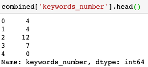

Few movies do not have a keywords value, some have more than one value. The helper function will parse only the first 3 keywords (if exist) and create 3 new columns named: ‘key1’, ‘key2’, ‘key3’ in the combined dataset.

def parse_keywords(x):
    if type(x) == str:
        return pd.Series(['','',''], index=['key1', 'key2', 'key3'])
    if len(x) == 1:
        return pd.Series([x[0]['name'],'',''], index=['key1', 'key2', 'key3'])
    if len(x) == 2:
        return pd.Series([x[0]['name'],x[1]['name'],''], index=['key1', 'key2', 'key3'])
    if len(x) > 2:
        return pd.Series([x[0]['name'],x[1]['name'],x[2]['name']], index=['key1', 'key2', 'key3'])

Apply the function to create 3 new columns and drop the original ‘Keywords’ column:

combined[['key1', 'key2', 'key3']] = \
        combined['Keywords'].apply(parse_keywords)
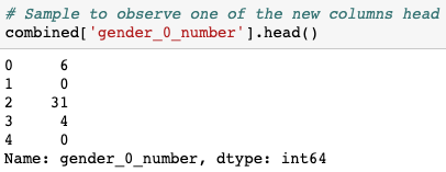
combined.drop(columns='Keywords', inplace=True)

Create 3 new features. Counting the number of the cast for genders 0,1,2 for each movie.

combined['gender_0_number'] = combined['cast'].apply(lambda row: sum([x['gender'] == 0 for x in row]))
combined['gender_1_number'] = combined['cast'].apply(lambda row: sum([x['gender'] == 1 for x in row]))
combined['gender_2_number'] = combined['cast'].apply(lambda row: sum([x['gender'] == 2 for x in row]))

Sample to observe one of the new columns head:

Create a new column with the number of cast values for each movie with the code-line:

combined['cast_number'] = \
        combined['cast'].apply(lambda x: len(x))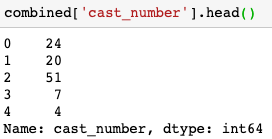

Parsing the cast column. Taking the first five cast members by their cast_id values and creating five cast-related new columns:

def parse_cast(x):
    myindx = ['cast1', 'cast2', 'cast3', 'cast4', 'cast5']
    out = [-1]*5
    if type(x) != str:
        for i in range(min([5,len(x)])):
            out[i] = x[i]['id']
    return pd.Series(out, index=myindx)

Apply the function to create 5 new columns and drop the original ‘cast’ column:

combined[['cast1', 'cast2', 'cast3', 'cast4', 'cast5']] = combined['cast'].apply(parse_cast)
combined.drop(columns='cast', inplace=True)

Create a new column with the number of crew values for each movie:

combined['crew_number'] = \
        combined['crew'].apply(lambda x: len(x))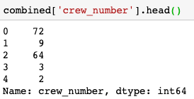

A function to parse the Director and Producer from the ‘crew’ column:

def parse_crew(x):
    myindx = ['Director', 'Producer']
    out = [-1]*2
    if type(x) != str:
        for item in x:
            if item['job'] == 'Director':
                out[0] = item['id']
            elif item['job'] == 'Producer':
                out[1] = item['id']
    return pd.Series(out, index=myindx)

Apply the function to create 2 new columns and drop the original ‘crew’ column:

combined[['Director', 'Producer']] = combined['crew'].apply(parse_crew)
combined.drop(columns='crew', inplace=True)

Create two new columns (features) for the two columns that contain Numeric Values (‘budget’, ‘popularity’) using np.log1p (calculate log(1 + x)) since there is a possibility that we will have a zero value and log of zero does not exist. RandomForest or light_gbm models can use both features without a conflict, Moreover, these two new features contribute to the models’ accuracy.

combined['budget_log'] = np.log1p(combined['budget'])
combined['pop_log'] = np.log1p(combined['popularity'])

Apply LabelEncoder on the new 5 generated feature-groups columns, fit and transform as a second step.

cols = ['genres1', 'genres2', 'genres3']
allitems = list(set(combined[cols].values.ravel().tolist()))
labeler = LabelEncoder()
labeler.fit(allitems)
combined[cols] = combined[cols].apply(lambda x: labeler.transform(x))

cols = ['prod1', 'prod2', 'prod3']
allitems = list(set(combined[cols].values.ravel().tolist()))
labeler = LabelEncoder()
labeler.fit(allitems)
combined[cols] = combined[cols].apply(lambda x: labeler.transform(x))

cols = ['country1', 'country2', 'country3']
allitems = list(set(combined[cols].values.ravel().tolist()))
labeler = LabelEncoder()
labeler.fit(allitems)
combined[cols] = combined[cols].apply(lambda x: labeler.transform(x))

cols = ['lang1', 'lang2', 'lang3']
allitems = list(set(combined[cols].values.ravel().tolist()))
labeler = LabelEncoder()
labeler.fit(allitems)
combined[cols] = combined[cols].apply(lambda x: labeler.transform(x))

cols = ['key1', 'key2', 'key3']
allitems = list(set(combined[cols].values.ravel().tolist()))
labeler = LabelEncoder()
labeler.fit(allitems)
combined[cols] = combined[cols].apply(lambda x: labeler.transform(x))

Apply Label Encode the two left category column:

combined_dummy = combined.copy()
cat_col = combined.select_dtypes('object').columns
combined_dummy[cat_col] = combined_dummy[cat_col].apply(lambda x: LabelEncoder().fit_transform(x))

Split the combined dataset back to Test and Train sets

train_data = combined_dummy.iloc[:ntrain]
test_data = combined_dummy.iloc[-ntest:]

Another three steps of preparation:

# Drop the 'revenue' column, it is the values to predict 
X_train = train_data.drop(columns='revenue').values

# The log transformation of the revenue gives better results, hence, we will use it
y_train = np.log1p(train_data['revenue'].values)

# Drop the 'revenue' column, will be filled at the end when the model will be ready
X_test = test_data.drop(columns='revenue').values

Model Building

Start with a basic Linear Regression Model.

kf = KFold(n_splits=5, shuffle=True, random_state=123)
lr = LinearRegression()
y_pred = cross_val_predict(lr, X_train, y_train, cv=kf)
y_pred[y_pred < 0 ] = 0

Continue with a random forest regression model (Improved result comparing to the LinearRegression try).

rf = RandomForestRegressor(max_depth=20, random_state=123, n_estimators=100)
y_pred = cross_val_predict(rf, X_train, y_train, cv=kf)
y_pred[y_pred < 0 ] = 0

View the importance of the features of the random forest model in a bar plot. dropping the revenue column before.

rf.fit(X_train, y_train)
imp = pd.Series(rf.feature_importances_, index=train_data.drop(columns='revenue').columns)
imp.sort_values(ascending=False).plot(kind='barh', figsize=(8,10))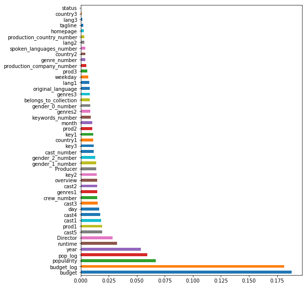

Continue with a LGBMRegressor Model (fast execution) the results improved comparing to the RandomForestRegressor try. The parameters of this model explanation: 0.4 means that for each of the 1500 (n_estimator) only 40% of the features will be selected (randomly). max_depth is inf (-1) but is restricted by the leaves number (20).

lgb_model = lgb.LGBMRegressor(num_leaves=20, max_depth=-1, learning_rate=0.01, 
                              metrics='rmse', n_estimators=1500, feature_fraction = 0.4)

y_pred = cross_val_predict(lgb_model, X_train, y_train, cv=kf)

View the importance of the features of the LGBMRegressor model in a bar plot. Dropping the revenue column before According to this model, the year is the most important feature in predicting the revenue and that makes sense, as the years pass the revenue increase. (across all Industries) The second important feature according to this model is the production company, budget, director.. The choices of this model are relevant and lead to a better prediction outcome, compare to the previous two models that I tried.

lgb_model.fit(X_train, y_train)
imp = pd.Series(lgb_model.feature_importances_, index=train_data.drop(columns='revenue').columns)
imp.sort_values(ascending=False).plot(kind='barh', figsize=(8,10))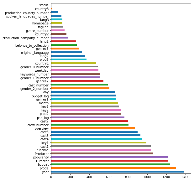

License

I open-sourced this jupyter-notebook for all to use as an entry point to the competition. If you, however, make progress and develop a better performance model, please let me know, empowering me to understand better and grow. Thank you. Ronnen.

This article, along with any associated source code and files, is licensed under GPL. (GPLv3)

← Previous Post