Introduction
The MNIST database of handwritten digits has a training set of 60,000 examples, and a test set of 10,000 examples. It is a subset of a larger set available from NIST. The digits have been size-normalized and centered in a fixed-size image.
Background
The original black and white (bilevel) images from NIST were size normalized to fit in a 20x20 pixel box while preserving their aspect ratio. The resulting images contain grey levels as a result of the anti-aliasing technique used by the normalization algorithm. the images were centered in a 28x28 image by computing the center of mass of the pixels, and translating the image so as to position this point at the center of the 28x28 field.
With some classification methods (particularly template-based methods, such as SVM and K-nearest neighbors), the error rate improves when the digits are centered by bounding box rather than center of mass.
The Challenge
The challenge in this task divided into 4 parts, followed by specific instructions. My full Solution written in Python Jupyter-Notebook can be downloaded directly.
The beginning of the task:
from scipy import io
from sklearn.model_selection import train_test_split

#the downloaded file
data = io.loadmat('mnist-original.mat')

#the data
x, y = data['data'].T, data['label'].T
x_train, x_test, y_train, y_test = train_test_split(x, y, test_size=0.5)
Part I
Preprocess the data. Visualize one element from each class. Visualize the mean of each class.
My solution included Looping over X_images and y_train ten times (for each class/digit) and Looking for the index (named ‘location’) in y_train, then extracting one of the proper figures from X_images.
plt.figure(figsize=(12,5))

for i in range(10):
    plt.subplot(2,5,i+1)
    location = np.where(y_train == i)[0][0] # find the first location of every class (digit)
    plt.imshow(X_images[location]) # plot a sample for each class (digit) according to the location
    plt.title(f'Number: {y_train[location]}')
    plt.xticks([]) # Remove the x,y-axis labels (not relevant, the 28X28 size is known)
    plt.yticks([])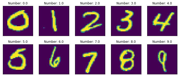
My Solution for the means visualization started with combining X_image, y_train into a zipped list. The zipped list contain pairs of: one item from X_images, and one item from y_train.
The second part of my solution include Building a new dictionary with a loop over the zipped list. The new dictionary will be used later for the means calculations.
The last part include Looping and plotting the mean of every class (digit).
zipped_data = list(zip(X_images, y_train))

zipped_dict = {}

for x,y2 in zipped_data:
    if y2 not in zipped_dict.keys(): # if the key is not exists, create it
        zipped_dict[y2] = [x]
    else:
        zipped_dict[y2].append(x) # if the key exists, append it to the relevant class

#Loop and plot the mean of every class (digit)

plt.figure(figsize=(12,5))

for i in range(10):
    plt.subplot(2,5,i+1)
    plt.imshow(np.mean(zipped_dict[i], axis=0)) # Plot the mean of each class (digit)
    plt.title(f'mean of: {i}')
    plt.xticks([]) # Remove the x,y-axis labels (not relevant, the 28X28 size is known)
    plt.yticks([])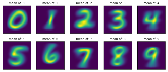
Part II
Try fitting a logistic regression with its solver set to be the ‘Ibfgs’ algorithm. (If you’d like, you can try the other solvers/optimizers and observe the differences in computation time.)
What does reducing the dimensionality do to the computation time and why? What does reducing the number of data points do to the computation time and why? List one advantage and disadvantage of reducing dimensionality. List one advantage and disadvantage of reducing the number of data points.
My Solution: This is a multiple class case using a Logistic Regression model; hence, the binary model creates a separate model for each class and choose the best one for the prediction, according to probabilities. (This is the disadvantage of using Logistic Regression model on multiple classes)
%%time

# Changed to multi_class='ovr' following the warnings for multi_class

log = LogisticRegression(solver='lbfgs', multi_class='ovr')
log.fit(X_train, y_train)
print(log.score(X_test, y_test))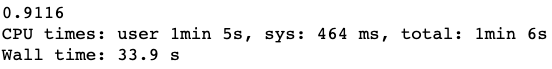
Reducing the dimensionality by slicing and reducing the number of columns, the computation time is (naturally) lower since we reduced the data size. The reason is that we working now on a smaller dataset.
%%time
#reducting number of columns

log = LogisticRegression(solver='lbfgs', max_iter=100, multi_class='ovr')
log.fit(X_train[:,:350], y_train)
print(log.score(X_test[:,:350], y_test))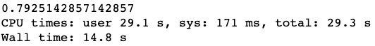
Reducing the number of data points reduce the computation time as well, for the same reason, the solver works on a lower number of data points. Hence, the computation time is shorter and the accuracy is lower too.
%%time
#reducing number of data points

log = LogisticRegression(solver='lbfgs', multi_class='ovr')
log.fit(X_train[:100], y_train[:100])
print(log.score(X_test[:100], y_test[:100]))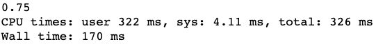
one advantage for reducing dimensionality: a faster computation time. one disadvantage for reducing dimensionality: we can miss some essential columns from the data resulting in a non-accurate model. However, if we reduce the number dimensionality by reducing the components as an output of the PCA method, that way, we reduce the dimensionality and focus on the most critical components.
one advantage of reducing the number of data points: A faster computation time. one disadvantage of reducing the number of data points: if we do that without planning and thinking in advanced, we can (randomly) reject essential points from the dataset.
Part III
Use 5-fold cross-validation with a KNN classifier to model the data. Try various values of k (e.g. from 1 to 15) to find the ideal number of neighbors for the model. What kind of accuracy are you getting? If you find this is taking too long for your computer you can subset the data to reduce the number of training points. What happens to train and validation set accuracy if you set the K in your K-NN model to 1 (1-Nearest Neighbours) or to the number of training points (60000-Nearest Neighbours). Can you explain what is going on and why it is happening? Answer the previous question again but using decision trees where instead of controlling for K we control for the depth of the tree.
My Solution: 5-fold cross validation divides the data into five parts, train on 4 slices and test it on the last one. That will happen five times (5 combinations of the split)
The loop ideally runs for each value between 1~15 and plots at the end the ideal number of neighbours for the model.
This is not a full run since a full run takes a long run-time. (did not complete after 24 hours)
Hence, the choice is a randomly chosen 1000 out of the all, a portion of the dataset that runs in a reasonable run-time. the accuracy here at the pick point (around 5 neighbors) is close to 87%.
#Randomly select a subset of data
#Generating a 1000 random numbers between 0 to X.shape[0]
indx = np.random.randint(0, X.shape[0], 1000)

#5 splits, random_state for my internal comparison
kf = KFold(n_splits=5, random_state=123)

#Array that will append the scores
scores_neighbors = []

for n in range(1,16):
    knn = KNeighborsClassifier(n_neighbors=n)
    scores = cross_val_score(knn, X[indx], y[indx], cv=kf)
    scores_neighbors.append(scores.mean())
plt.plot(range(1,16), scores_neighbors)
plt.xlabel('number of neighbors')
plt.ylabel('accuracy')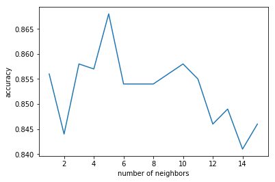
What happens to the accuracy if you set the K in KNN to 1?
Setting K=1 will give 100% accuracy if the model will be trained on the all dataset since we will always find one that is the closest to itself, in a case of a train set as a portion, the accuracy will not be 100% on the test set.
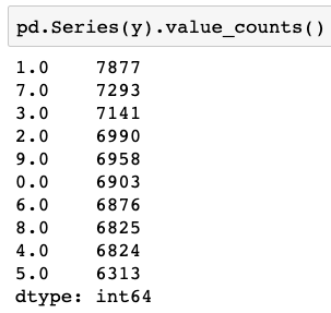
What will happens to the accuracy if you set the k in KNN to 60000?
How many we have from each class? Creating a pd on y (below) reveals that there are more from class ‘1’ compared to any other class. Hence, Setting 60000 near neighbours, the highest value is ‘1’ so the algo will always choose ‘1’ in this case to classify the point, the class with the highest number of images.
Changing to decision trees and looping over the depth of the tree reveals a graph that shows a good result in depth 10, from 10 forwards the accuracy became slightly lower.
#randomly select a subset of data
np.random.seed(123)

#Generating 10000 random points
indx = np.random.randint(0, X.shape[0], 10000)

kf = KFold(n_splits=5, random_state=123)

scores_tree = []

for n in range(1,25):
    tree = DecisionTreeClassifier(max_depth=n)
    scores = cross_val_score(tree, X[indx], y[indx], cv=kf)
    scores_tree.append(scores.mean())

plt.plot(range(1,25), scores_tree)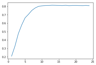
Part IV
Fit a linear model, such as logistic regression or an SVM (to speed up training you can modify the default settings). Try to get as high an accuracy as possible on a validation set. What does the class confusion matrix look like for your best model? Is there anything that stands out in it? Re-fit a linear model that can discriminate between the digit 4 and the digit 9. Visualize the weights of the model as an image, does anything stand out?
My Solution: Starting with a Logistic Regression Model.
#A Logistic Regression model
log = LogisticRegression(solver='lbfgs', multi_class='ovr')
log.fit(X_train, y_train)
print(f'The score is: {log.score(X_test, y_test)}')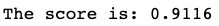
Here I created a second y_predict = log.predict(X_test) and passed it into the matrix, with the real value. (y_test)
y_pred2 = log.predict(X_test)
pd.DataFrame(confusion_matrix(y_test, y_pred2),
             columns=range(10), index=range(10))
The diagonal line in the Confusion Matrix stands out, the values are higher compared to the others. The higher values related to our (relatively) high score.
Other than the diagonal, the Inaccuracies values are relatively low, at column 8 row 2 there is an Inaccuracy of 119 for example.
Regarding the question: Re-fit a linear model that can discriminate between the digit 4 and the digit 9 and visualise, I Created a variable that will contain only True and False for the relevant digits: 4 and 9:
indx49 = np.logical_or(y_train == 4, y_train == 9)
log = LogisticRegression(solver='lbfgs')
# partial fit, only on the 4 and 9 digits
log.fit(X_train[indx49] , y_train[indx49])
# The plot
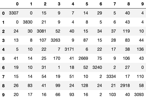
plt.imshow(log.coef_.reshape(28,28))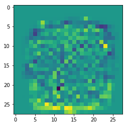
Interpretation: The yellow dots on the bottom (mainly) imply a magnitude values, these are the points that the algorithm can distinguish between the values 4 and 9.
There is no presentation to both digits at the bottom, where some of the yellow points located.
Part V
Your goal is to train a model that maximizes the predictive performance (accuracy in this case) on this task. Optimize your model’s hyperparameters if it has any. Give evidence why you believe the hyperparameters that you found are the best ones. Provide visualizations that demonstrate the model’s performance.
My Solution: Starting with a Logistic Model, the hyperparameters there are the regularisation penalty values (and others), but the run time is slow, and I’m not sure that Logistic is the right fit for this model.
Another try made with KNN model, the run time delays the flow of the work.
So, the choice here was to train a decision tree, starting with the hyperparameters best values (for few selected hyperparameters), continue with splitting the train portion into a train and validate portions. In the case of a decision tree, the validation portion will help to asses the optimal Depth of the tree.
#Starting again with the basic steps for practice.
#Split into two subgroups, 50% for each
X_train, X_test, y_train, y_test = train_test_split(X, y, test_size=0.5)

#Fit and Transform
scaler  = StandardScaler()
X_train = scaler.fit_transform(X_train)
X_test  = scaler.transform(X_test)
I started with SOME Hyperparameters Tuning for a decision tree, Setup the parameters and the distributions to sample, from: param_dist
#SOME Hyperparameters Tuning for a decision tree
#Setup the parameters and the distributions to sample, from: param_dist

param_dist = {
                "max_depth": [3, None],
                "min_samples_leaf": [2,4],
                "criterion": ["gini", "entropy"]
             }

#Instantiate a tree classifier object
tree = DecisionTreeClassifier()

#Trigger the GridSearchCV function
tree_cv = RandomizedSearchCV(tree, param_dist)

#Fit the data
tree_cv.fit(X_train, y_train)

#Print the results
print(f'The tuned decision tree parameters: {tree_cv.best_params_}')
print(f'The best score is: {tree_cv.best_score_}')
There are few hyperparameters for a decision tree, we found the best value for few of them (some combination) with an exception for the max_depth (returns ‘None’), hence another check is needed.
I created a prediction for the test set results and continued with Visualizing the results with a confusion matrix with the code:
#Predict the test set results
y_pred = tree_cv.predict(X_test)

#Visualizing the results with a confusion matrix
plt.figure(figsize=(12,8))
pd.DataFrame(confusion_matrix(y_test, y_pred),
                 columns=range(10), index=range(10))
The outcome Confusion Matrix:
The confusion matrix values are normal for this kind of accuracy, the diagonal values are the highest, with relatively low values else that relates to model Inaccuracies.
The max_depth value output from the previous step is not satisfying, hence another run and plot are needed to evaluate the optimal value of the depth. Start with another split, a split of the train into: train, validate.
#Split X_train, y_train into two subgroups: train and validate, 50% each
X_train, X_validate, y_train, y_validate = \
                    train_test_split( X_train, y_train, test_size=0.5 )

scaler  = StandardScaler()

#Fit and Transform
X_train     = scaler.fit_transform(X_train)
X_validate  = scaler.transform(X_validate)


np.random.seed(123)
indx = np.random.randint(0, X.shape[0], 1000)

kf = KFold(n_splits=5, random_state=123)

#Arrays that will hold the accuracy results
acc_validate = []
acc_train    = []

#The function 'cross_validate' returns a dictionary
#my_dict will catch it
my_dict = {}

for n in range(1,20, 1):

    tree = DecisionTreeClassifier( max_depth=n )

    my_dict = cross_validate( tree, X[indx], y[indx], cv=kf ,\
                                            return_train_score=True )

    acc_train.append( my_dict['train_score'].mean() )
    acc_validate.append( my_dict['test_score'].mean() )
Plot the accuracy scores of the train portion along the validation portion scores:
plt.figure()
plt.plot(range(1,20, 1), acc_train, label='train')
plt.plot(range(1,20, 1), acc_validate, label='validate')
plt.xticks(range(1,20, 1))
plt.xlabel('Tree Depth')
plt.ylabel('Accuracy')
plt.legend()
plt.show()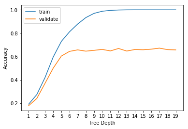
From the plot we can see that Depth 5 Looks like an appropriate point, and higher values can lead to overfitting.
Accourding to the results, I decided to build a Model with the combination of hyperparameters as follow:
DT_model = DecisionTreeClassifier( max_depth=5, \
                                   min_samples_leaf=2, \
                                   criterion='entropy' )
DT_model.fit(X_train, y_train)
License
This article, along with any associated source code and files, is licensed under GPL. (GPLv3)